|
|
 |
National Weather Service |
 |
|
| National Operational Hydrologic Remote Sensing Center |
| Home | News | Organization |
|
NOHRSC Technology > NOHRSC GIS Applications > Unit Hydrograph Unit Hydrograph (UHG)
|
||||||||||||||||||||||||||||||||||||||||||||||||||||||||||||||||||||||||||||||||||||||||||||||||||||||||||||||||||||||||||||||||||||||||||||||||||||||||||||||||||||||||||||||||||||||||||||
|
|
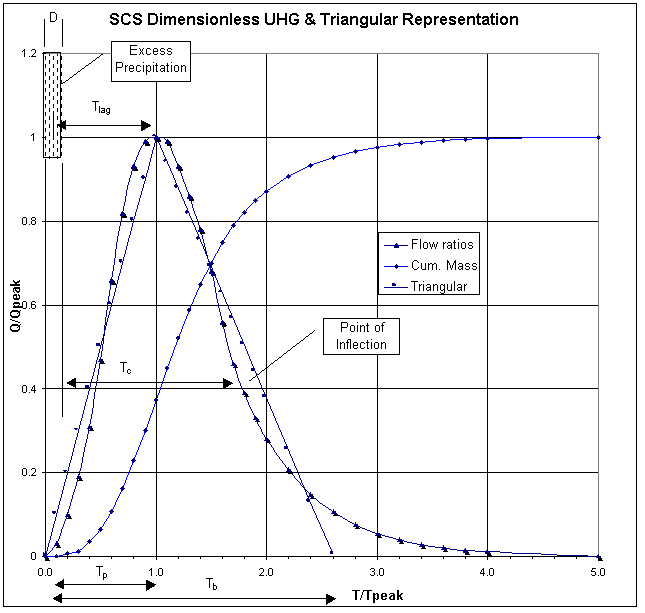
Figure 2 - Illustration of dimensionless curvilinear unit hydrograph and equivalent triangular hydrograph.
The volume, Q, is in inches (1 inch for a unit hydrograph) and the time is in hours. The peak rate, qp, in inches per hour, is found to be :
![]() Equation 4
Equation 4
It is desirable to have the peak flow of the unit hydrograph in terms of cfs per inch per square mile of drainage area. To accomplish this, the term, qp, in the above equation is converted to cubic feet per second and the drainage area, A (mi2), is brought into the equation, which results in an equation of expressing the runoff per inch per square mile:
![]() Equation 5
Equation 5
The 645.33 is the conversion used for delivering 1-inch of runoff (the area under the unit hydrograph) from 1-square mile in 1-hour (3600 seconds). Noting again that the recession limb time, Tr, is 1.67 times the time to peak, Tp. Substituting in these relationships from Equation 1 above, Equation 5 is rewritten:
![]()
![]() Equation 6
Equation 6
Because the above relationships were developed based on the volumetric constraints of the triangular unit hydrograph, the equations and conversions are also valid for the curvilinear unit hydrograph, which, proportionally, has the same volumes as the triangular representation. The conversion constant (herein called the peaking factor) 484 is the result of the large number of unit hydrographs from a wide range of basin characteristics and actually reflects the ability of the watershed to retain and delay the flow. Note that the value 484 is the result of assuming that the recession limb is 1.67 time the rising limb (time to peak). This may not be applicable to all watershed types.
Steep terrain and urban areas may tend to produce higher early peaks and thus values of the peaking factor may tend towards 600. Likewise, flat swampy regions tend to retain and store the water, causing a delayed, lower peak. In these circumstances values may tend towards 300 or lower (SCS 1972; Wanielista, et al. 1997). It would be very important to document any reasons for changing the constant from 484, effectively changing the shape of the unit hydrograph. When changing the shape of the unit hydrograph, one must keep in mind the ratios of the volumes under the rising and recession sides of the original dimensionless unit hydrograph and the resulting volume under the unit graph must remain at 1 inch. More information concerning the peak factor estimation is provided in "SCS Parameter Estimation", below.
The peak rate may also be expressed in terms of other timing parameters besides the time-to-peak. From Figure 2:
![]() Equation 7
Equation 7
where D = the duration of the unit excess rainfall and L = the basin lag time, which is defined as the time between the center of mass of excess rainfall and the time to peak of the unit hydrograph. The peak flow is now written as:
 Equation 8
The SCS (1972) relates the lag time, L, to the time of concentration, Tc by :
![]() Equation 9
Equation 9
Combining this with other relationships, as illustrated in the triangular unit hydrograph, the following relationships develop:
![]() Equation 10
Equation 10
and
![]() Equation 11
Equation 11
From this, the duration D may be expressed as:
![]() Equation 12
Equation 12
Equations 1 through 10 provide the basis for the SCS Dimensionless Unit Hydrograph method in UHG. Equation 12 provides a desirable relationship between duration and time of concentration, which should provide enough points to accurately represent the unit hydrograph, particularly the rising limb.
It is necessary to estimate the area and a timing parameter for construction of the SCS unit hydrograph. In addition, the peaking factor, which defaults to 484 may be altered by the user. BUGHTool calculates a triangular unit hydrograph. This was done for several reasons, the main being that while the original SCS method provides dimensionless values for a curvilinear unit hydrograph, there are no dimensionless values for unit hydrographs that peak earlier or later. In other words, if a peaking factor other than 484 is used (see Equation 6), then the resulting unit hydrograph would require new dimensionless flow and timing ratios.
Area
Suffice it to say that the drainage area, A, should be obtained with as much accuracy and precision as is possible. Within the context of the planned implementation at RFC's, the area already have been estimated as part of IHABBS. For the basins typically to be encountered by the RFCs and WFOs, the 15-arc second data should provide areas within a few percent. Rost (1998) found that the 15-arc second data used in both IHABBS and UHG is capable of accurately delineating basins that are well below 50 square kilometers (20 square miles).
Peaking Factor
The "peaking factor" essentially controls the volume of water on the rising and recession limbs. The default value is 484 as illustrated in the original derivation and Equation 6. This is; however, a user option in UHG when using the SCS method. Table 2 provides some guidance for the selection of this parameter.
Table 2 - Hydrograph peaking factors and recession limb ratios (Wanielista, et al. 1997)
| General Description | Peaking Factor |
Limb Ratio (Recession to Rising) |
| Urban areas; steep slopes | 575 | 1.25 |
| Typical SCS | 484 | 1.67 |
| Misxed urban/rural | 400 | 2.25 |
| Rural, rolling hills | 300 | 3.33 |
| Rural, slight slopes | 200 | 5.5 |
| Rural, very flat | 100 | 12.0 |
Timing
The timing parameter is somewhat difficult to estimate and rather subjective, however; this parameter has considerable influence on the values of the unit hydrograph. Underestimating the unit hydrographs "timing" will cause the peak to occur earlier and higher, while over estimating will cause a delayed and lower peak. There are several methods for estimating the timing parameter in UHG. These methods are discussed in detail below.
SCS Lag Equation
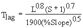
The SCS lag equation is an empirical approach developed by the SCS, which estimates lag time directly. The SCS (1972) also recommends that the lag equation be used on basins that may be considered somewhat homogeneous in nature and less than 2000 acres in size. Due to these restrictive recommendations, the method may be rather limited in application to most of the basins which are typically encountered in the daily forecasting operations of the NWS; however, due to the relative ease of estimation and the potential for having smaller basins, this method will be included. Restrictions on the use of the lag equation should be stated, although some leeway beyond the 2000 acres size limit may be justifiable. The SCS lag equation is given as:
 Equation 13
where : Tlag = lag time in hours
L = Length of the longest drainage path in feet
S = (1000/CN) - 10
CN =curve number
%Slope = The average watershed slope in %
It will also be necessary to derive the average SCS curve number (CN). At the present time, the curve number is a user input; however, the average curve number for the basin will be computed using a raster curve number data layer.
The remaining parameters are the Length, L, and the % Slope. The length, L is the length of the longest drainage path from the watershed outlet to the watershed divide, which is generally obvious for most watersheds. The length is calculated using the 15-arc second flow direction grid, which was included in the IHABBS installation. Each cell's flow path is traced to basin outlet and the longest flow (by distance) is noted and recorded.
The somewhat more difficult parameter is the slope. The slope is calculated from a 15-arc second slope data set. The difficulty in using an average slope is the possibility of non-contributing areas being used in the average slope calculation. For example, areas very near the stream may be somewhat steep and be the main source of contributing area to a runoff hydrograph, while the land farther away from the stream may be a mild sloping plateau that does not readily contribute to the basin response. The effect would be to include the mild sloping cells in the average slope calculation, producing a mild average slope and a lower peaking, longer lag time unit hydrograph.
Segmental Approaches
In the segmental velocity or segmental approach, the parameter being estimated is essentially the time of concentration or longest travel time within the basin. In general, the longest travel time corresponds to the longest drainage path; however, there may be situations and basin configurations that allow for some shorter travel distances to have longer travel times, due to land use and/or flow type. As in the case of the SCS lag equation, each grid cell's flow is traced to the basin outlet and the travel time across each downstream grid cell en route to the outlet is calculated. The sum of all of the travel times represents the time of concentration. Equation 7 is then used to estimate the lag time for use in calculating the SCS dimensionless unit hydrograph. Under the segmental approach, there are several options for estimating the travel time across each cell, which are described in the following sections.
Constant velocity
The constant velocity method is a very simplistic approach that allows the user to assign a constant velocity to all grid cells. Again, the flow path of cell is traced to the basin outlet and travel times across each grid cell are summed to estimate the longest travel time. The user must supply the constant velocity.
Land Use Based
This option will not be available in the first release, however; a description of the planned implementation is provided. Travel times are calculated for each grid cell using an equation of the following form to calculate velocities:
![]() Equation 14
Equation 14
Where k is a coefficient based on the particular land use. The travel length across the cell divided by the velocity (time = distance/velocity) provides an estimate of the travel time. McCuen (1989) and SCS (1972) provide values of k for several land uses. Table 3 provides values of k for various land uses. A land use grid layer will be eventually be deployed, which will provide similar land use types and corresponding k values as illustrated in Table 3.
Table 3 - Coefficients of velocity (fps) versus slope (%) relationship for estimating travel velocities (McCuen 1989; SCS 1972).
| K | Land Use / Flow Regime |
| 0.25 | Forest with heavy ground litter, hay meadow (overland flow) |
| 0.5 | Trash fallow or minimum tillage cultivation; contour or strip cropped; woodland (overland flow) |
| 0.7 | Short grass pasture (overland flow) |
| 0.9 | Cultivated straight row (overland flow) |
| 1.0 | Nearly bare and untilled (overland flow); alluvial fans in western mountain regions |
| 1.5 | Grassed waterway |
| 2.0 | Paved area (sheet flow); small upland gullies |
Flow Type Based
This method is very similar to the "Land Use Based" method, however; instead of land use categories, the velocity is based on an assumed flow type. The three flow types are overland flow, swale flow, and channel flow. Travel times are calculated for each grid cell using an equation of the form:
![]() Equation 15
Equation 15
Where k is a coefficient based on the flow type. The Michigan Department of Natural Resources - Land and Water Management Division ((Sorrell and Hamilton 1991) provide relationships, as illustrated in Table 4.
Table 4 - Coefficients of velocity (fps) versus slope (%) relationship for estimating travel velocities (Sorrell and Hamilton 1991).
| Flow Type | K |
| Small Tributary - Permanent or intermittent streams which appear as solid or dashed blue lines on USGS topographic maps. | 2.1 |
| Waterway - Any overland flow route which is a well defined swale by elevation contours, but is not a stream section as defined above. | 1.2 |
| Sheet Flow - Any other overland flow path which does not conform to the definition of a waterway. | 0.48 |
Flow type is determined within UHG in the following manner. Overland flow is considered to exist for a "short distance" on all cells that have no upstream cells (i.e. the ridge top cells). The "short distance", which defaults to 50 meters (~164 feet), is also a user option ranging between 0 and 100 meters (0 to 328 feet). Swale flow is then considered to exist until a channel cell is reached. Channel cells are defined in one of two ways in UHG.
First, the user may opt to use the EPA river reach files (RF1) which are included in the installation of IHABBS. Any cell that coincides with a river cell is considered to be a channel cell and the appropriate coefficient, k is applied. The alternative method is to use the flow accumulation data layer to define the channel cells. In this option, the user selects a threshold accumulation value, which essentially states that any cell having a flow accumulation greater than the threshold value is considered to be a channel cell. The threshold runoff value is easily described by attempting to estimate how much drainage area is required before a stream channel is formed.
The best method of assigning this threshold parameter is to first look at USGS topographic maps and other sources of "local" data and determine the extent of the first order streams in an area. The location of the "tips" of these first order streams should then be located on one of the UHG raster data images. The user may "query" raster layers and determine the flow accumulation value at the 'heads" of several first order streams. This flow accumulation value can then be used in UHG to establish channel flow cells.
Flow Accumulation Based
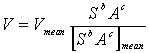
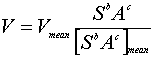
Maidment et al. (1994) provide the basis for this method, where velocity is calculated:
 Equation 16
Where V = the velocity of the cell, Vmean = the mean velocity in the basin, S = slope, A = upstream drainage area, and a and b are coefficients. Equation 13 can be rearranged into:
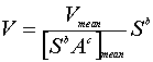 Equation 17
and allowing :
 Equation 18
then Equation 18 essentially becomes the same as Equations 14 and 15. In the UHG application, the denominator of Equation 18 is easily calculated using the flow direction grid, the flow accumulation grid, and the slope grid data layers. The more difficult of the parameters is the "mean velocity" or Vmean. In this version of UHG, the mean velocity will be a user input parameter.
Triangular Shape
UHG calculates a triangular shaped unit hydrograph and there is some concern about the ability of this shape to be used in an operational setting. In general, it can be said that the triangular version will not cause or introduce noticeable differences in the simulation of a storm event, particularly when one is concerned with the peak flow. For long term simulations, the triangular unit hydrograph may have potential impacts; however, due to the uncertainties in the "exact" dimensionless ratios, which would be needed for a curvilinear unit hydrograph, it has been decided to use the triangular function.
In order to account for concerns arising over the shape of the triangular version, the option to fit a gamma distribution has been added. Aron and White (1982) fitted a gamma probability distribution using peak flow and time to peak data. The gamma distribution is:
![]() Equation 19
Equation 19
McCuen (1989) provides a procedure for implementation of this method:
Step #1 - Compute:
![]() Equation 20
Equation 20
where :
qp = peak flow in cfs
tp = time to peak in hours
A = drainage area in acres
Step #2 - Find the value of "a" from the following :
![]() Equation 21
Equation 21
Step #3 - The ordinates of the unit hydrograph are calculated from:
![]() Equation 22
Equation 22
Figure 3 illustrates the fitting of the gamma distribution to a triangular unit hydrograph.
Figure 3 - Gamma fitted distribution of a triangular unit hydrograph.
Time-area unit hydrograph theory establishes a relationship between the travel time and a portion of a basin that may contribute runoff during that travel time. Clark (1945) is one of early examples of this method. The U. S. Army Corps of Engineers at the Hydrologic Engineering Center (HEC 1996) provide a description of a modified time-area approach, known as the ModClark method, which is part of the recently released HEC-HMS computer model (HEC 199x).
In a time-area approach, the watershed is traditionally broken into areas of approximately travel time. These lines of equal travel time are known as isochrones. Figure 4 illustrates the breaking of a watershed into areas by isochrones. The mean travel time of each sub-area is calculated and the resulting time-area curve is produced. Most of the "time-area" methods utilize a common, basic approach in determining the final unit hydrograph. Summing the incremental areas and corresponding travel times (6 in Figure 4) enables the formation of a cumulative time-area curve. Thus, the total time can be thought of as the time of concentration of the watershed with 100% of the basin area being accounted for at the time of concentration.

Figure 4 - Hypothetical watershed divided into 6 areas of approximately equal travel time to the outlet. Corresponding accumulative time-area curve is also illustrated.
Each of the partial areas (between isochrones) responds in the time associated with that area. Therefore, the cumulative time-area curve is a summation of the individual areas. The contributions of the individual areas can be illustrated with a histogram. One can visualize a uniform depth of water (1" for a unit hydrograph) on each of the zones within the isochrones. The volume of water of each area reaches the outlet at the travel time associated with that area. This is effectively a volume over a time period, which is a flow. Figure 5 illustrates a time-discharge histogram associated with the hypothetical basin of Figure 4.
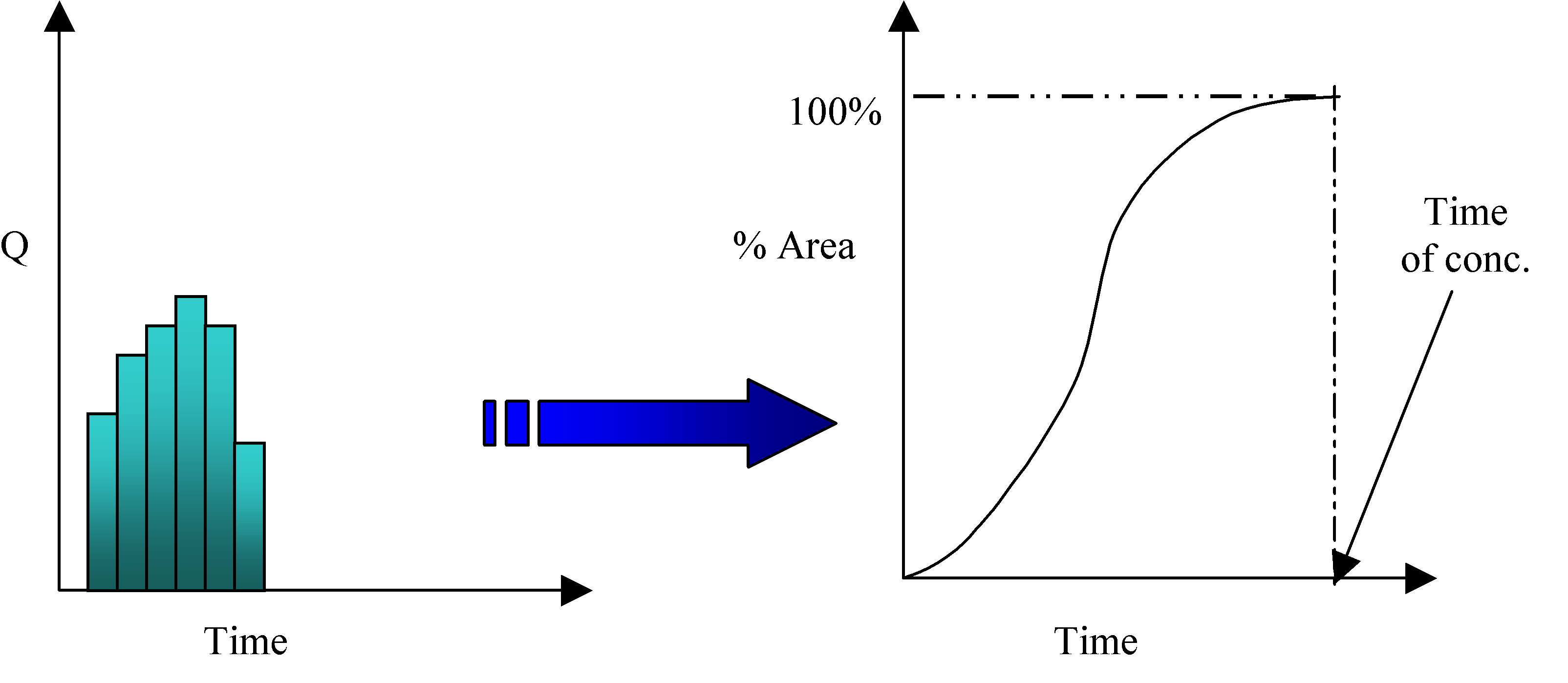
Figure 5 - Time-area histogram and associated cumulative time-area diagram.
The time-area histogram is really a translation hydrograph because the volume of water on each area within the basin is simply "translated" to the outlet using the associated travel time for the translation time. A this point, a unit hydrograph (in discrete form) exists. This "instantaneous" unit hydrograph is the result of 1-inch of instantaneous excess precipitation being placed on the individual areas and then translated to the outlet of the basin, arriving at the time associated with the travel time of area.
Watersheds also have the ability to store and delay the flow that passes through. This storage effect is seen in reservoirs as they attenuate a hydrograph. In order to model this effect, the translation unit hydrograph is routed through a linear reservoir. The concept of routing the translation unit hydrograph is illustrated in Figure 6.
Figure 6 - Illustration of translation unit hydrograph being routed through linear reservoir.
The instantaneous unit hydrograph (IUH) is then calculated by routing the translation unit hydrograph the linear reservoir, having a routing coefficient, R. This is accomplished by the following equation :
![]() Equation 23
Equation 23
where :
IUHi = ordinate of the instantaneous unit hydrograph
Ii = Value at time I of the translation unit hydrograph
and
![]() Equation 24
Equation 24
Where Dt = the time step used in the calculation of the translation unit hydrograph. The routed unit hydrograph is still considered to be an instantaneous unit hydrograph. A final unit hydrograph of a given duration can be found by lagging the instantaneous unit hydrograph by the desired duration and averaging the ordinates. The desired duration must be a multiple of the original time step employed in the computations above.
Within the time-area based approach, there are 3 different choices for "moving and delaying" the water en route to the basin outlet. Each of the methods uses the distributed nature of the raster data sets to varying degrees.
The first method is very similar to the ModClark method (HEC 1996). Each grid cell in the basin is assumed to have 1-inch of excess precipitation dropped on it instantaneously. This volume of water is then translated to the outlet and will arrive based on the cells known travel time to the outlet. The travel time to the outlet may be calculated in several ways itself, as in the SCS method described above. Once the water is translated to the outlet, it is grouped into an appropriate bin, which depends on the time interval of the computation. In other words, if the time interval is 1 hour and a cell arrives in 1.283 hours then that water is placed in the bin that spans hours 1 to 2. Likewise, a cell that arrives in 6.98 hours would have its volume of water placed in the bin spanning the hour 6 to 7, and so on.
This is basically the same as creating a cumulative time-area curve and desegregating into bins of the desired computation interval. Next the volume of water in each of the bins is then routed though a linear reservoir using Equation 20. The reservoir routing coefficient is the same for all bins (and grid cells) regardless of their location in the basin or time of arrival at the outlet. The method of estimating or determining the reservoir routing coefficient, R, is described below.
This time-area method is basically identical to the first, with the exception that each grid cell arrives at the outlet at its specified arrival time, however; the reservoir routing coefficient is dependant upon time it takes the cell to travel to the basin outlet.
The final method is somewhat more complicated. This method is thought of as a distributed unit hydrograph method, although that may sound like a contradiction in terms. The distributed method moves and delays the water across each cell as it travels to the basin outlet. Again, each cell is assumed to receive 1-inch of excess precipitation. This precipitation is routed off the cell on which it falls using a time-area method and breaking the cell into an equal number of isochrones of travel time. This is done for all cells. The water that leaves the cells is in the form a unit hydrograph for only one cell. The unit hydrograph for that cell is then lagged or translated across each downstream cell and routed through a linear reservoir on each cell. The lagging across each cell is dependent on the travel time across the cell and the reservoir routing is dependent on a reservoir routing coefficient, which is calculate for each cell. The lagging and routing continues downstream until the final hydrograph is tabulated at the outlet. This is a unit hydrograph that has resulted from lagging and routing 1-inch of excess precipitation throughout the watershed to the outlet in a distributed fashion.
This distributed method is not perceived by the authors to be necessary on all watersheds, as it will be most applicable on watersheds that have very complex topology and drainage patterns. Experience thus far indicates that the time to peak and the magnitude of the are not drastically different from other time-area methods; however, the distributed method has been able to capture subsequent peaks much better.
The basic parameters that are necessary to estimate are travel times, basin area, and a method of estimating the linear reservoir routing coefficient, R.
Area
Suffice it to say that the drainage area, A, should be obtained with as much accuracy and precision as is possible. Within the context of the planned implementation at RFC's, the area already have been estimated as part of For the basins typically to be encountered by the RFCs and WFOs, the 15-arc second data should provide areas within a few percent. Rost (1998) found that the 15-arc second data used in both IHABBS and UHG is capable of accurately delineating basins that are well below 50 square kilometers (20 square miles).
Linear Reservoir Coefficient Estimation
The linear reservoir coefficient is very difficult to estimate. The most appropriate and desirable method of estimation is to utilize stream flow data and estimate the parameter as previously discussed. Clark (1945) provided a means of estimating R by considering a measured hydrograph and calculating R by :
![]() Equation 25
Equation 25
where : Q, dq, and dt are measured at the inflection point on the recession limb of a hydrograph at the gauge site. The routing coefficient, R, may also be estimated by dividing the volume under the recession limb by the flow at the inflection point on the recession limb (HEC 1982). In ungauged basins, it is possible to estimate the reservoir routing coefficient from a nearby basin (or a nested basin) and apply it to the ungauged basin.
A second desirable method is to estimate the coefficient from a number of nearby basins and perform a linear regression analysis including such parameters as area, slope, channel information, etc.. With this in mind, it is obviously preferred that the user performs some type of analysis to estimate the linear storage parameter in some a priori manner for the basin or a nearby basin. In the absence of all other inputs, the longest travel time from the any cell to the basin outlet may be used to estimate the routing coefficient (Wanielista, Kerten, & Eaglin 1997). From experience and personal contact with other researchers and engineers, a value of 0.7 times the longest travel time may be used for the value of the linear routing coefficient. The user is able to change this multiplier.
Timing Estimates
All of the options in the segmental approach described above are again available for use with the time area approach. These methods are described in above and are provided here for completeness.
Segmental Approaches
In the segmental velocity or segmental approach, the parameter being estimated is essentially the time of concentration or longest travel time within the basin. In general, the longest travel time corresponds to the longest drainage path; however, there may be situations and basin configurations that allow for some shorter travel distances to have longer travel times, due to land use and/or flow type. As in the case of the SCS lag equation, each grid cell's flow is traced to the basin outlet and the travel time across each downstream grid cell en route to the outlet is calculate. The sum of all of the travel times represents the time of concentration. Equation 7 is then used to estimate the lag time for use in calculating the SCS dimensionless unit hydrograph.
Constant velocity
The constant velocity method is a very simplistic approach that is included in UHG . This method allows the user to assign a constant velocity to all grid cells. Again, the flow path is of cell is traced to the basin outlet and travel times across each grid cell is summed to estimate the longest travel time. The user must supply the constant velocity.
Land Use Based
This option will not be available in the first release, however; a description of the planned implementation is provided. Travel times are calculated for each grid cell using an equation of the form:
![]() Equation 14
Equation 14
Where k is a coefficient based on the particular land use. McCuen (1989) and SCS (1972) provide values of k for several land uses. Table 5 provides values of k for various land uses. A land use grid layer will eventually be included in the UHG installation.
Table 5 - Coefficients of velocity (fps) versus slope (%) relationship for estimating travel velocities (McCuen 1989; SCS 1972).
| K | Land Use / Flow Regime |
| 0.25 | Forest with heavy ground litter, hay meadow (overland flow) |
| 0.5 | Trash fallow or minimum tillage cultivation; contour or strip cropped; woodland (overland flow) |
| 0.7 | Short grass pasture (overland flow) |
| 0.9 | Cultivated straight row (overland flow) |
| 1.0 | Nearly bare and untilled (overland flow); alluvial fans in western mountain regions |
| 1.5 | Grassed waterway |
| 2.0 | Paved area (sheet flow); small upland gullies |
Flow Type Based
This method is very similar to the "Land Use Based" method, however; instead of land use categories, the velocity is based on an assumed flow type. The three flow types are overland flow, swale flow, and channel flow. Travel times are calculated for each grid cell using an equation of the form :
![]() Equation 15
Equation 15
Where k is a coefficient based on the flow type. The Michigan Department of Natural Resources - Land and Water Management Division ((Sorrell and Hamilton 1991) provide relationships, as illustrated in Table 6. The user has control of these values, although the default values are those listed in Table 6.
Table 6 - Coefficients of velocity (fps) versus slope (%) relationship for estimating travel velocities (Sorrell and Hamilton 1991).
| Flow Type | K |
| Small Tributary - Permanent or intermittent streams which appear as solid or dashed blue lines on USGS topographic maps. | 2.1 |
| Waterway - Any overland flow route which is a well defined swale by elevation contours, but is not a stream section as defined above. | 1.2 |
| Sheet Flow - Any other overland flow path which does not conform to the definition of a waterway. | 0.48 |
Flow type is determined within UHG in the following manner. Overland flow is considered to exist for a "short distance" on all cells that have no upstream cells (i.e. the ridge top cells). The "short distance", which defaults to 50 meters (~164 feet), is also a user option ranging between 0 and 100 meters (0 to 328 feet). Swale flow is then considered to exist until a channel cell is reached. Channel cells are defined in one of two ways in UHG.
First, the user may opt to use the EPA river reach files (RF1) which are included in the installation of IHABBS. Any cell that coincides with a river cell is considered to be a channel cell and the appropriate coefficient, k is applied. The alternative method is to use the flow accumulation data layer to define the channel cells. In this option, the user selects a threshold accumulation value, which essentially states that any cell having a flow accumulation greater than the threshold value is considered to be a channel cell. The threshold runoff value is easily described by attempting to estimate how much drainage area is required before a stream channel is formed.
The best method of assigning this threshold parameter is to first look at USGS topographic maps and other sources of "local" data and determine the extent of the first order streams in an area. The location of the "tips" of these first order streams should then be located on one of the UHG raster data images. The user may "query" raster layers and determine the flow accumulation value at the 'heads" of several first order streams. This flow accumulation value can then be used in UHG to establish channel flow cells.
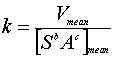
Flow Accumulation Based
Maidment et al. (1994) provide the basis for this method, which is based on the following equation:
 Equation 16
Where V = the velocity of the cell, Vmean = the mean velocity in the basin, S = slope, A = upstream drainage area, and a and b are coefficients. Equation 16 can be rearranged into:
Equation 17
and allowing :
Equation 18
then Equation 18 essentially becomes the same as Equations 14 and 15. In the UHG application, the denominator of Equation 18 is easily calculated using the flow direction grid, the flow accumulation grid, and the slope grid data layers. The more difficult of the parameters is the "mean velocity" or Vmean. In this version of UHG, the mean velocity will be a user input parameter.
Aron, G. and E. White, 1982. Fitting a Gamma Distribution Over a Synthetic Unit Hydrograph, Water Resources Bulletin, Vol. 18(1) 95-98, Feb. 1982.
Clark, C.O. 1945. "Storage and the Unit Hydrograph." Transactions of the American Society of Civil Engineers 110, pp. 1419-1446.
Hydrologic Engineering Center, 1982. Hydrologic Analysis of Ungauged Watersheds Using HEC-1, Training Document No. 15, U.S. Army Corps of Engineers, Hydrologic Engineering Center (HEC), Davis, CA.
Hydrologic Engineering Center, 1990. HEC-1 Flood Hydrograph Package, Program Users Manual, U.S. Army Corps of Engineers, Davis, CA.
McCuen, R. H. 1989. Hydrologic Analysis and Design. Prentice-Hall, Inc. Englewood Cliffs, NJ.
SCS, 1972 - (Soil Conservation Service). National Engineering Handbook, Section 4, U.S. Department of Agriculture, Washington, D.C.
Sorrell, Richard C. and David A Hamilton, 1991. Computing Flood Discharges for Small Ungaged Watersheds, Michigan Department of Natural Resources - Land and Water Management Division.
Wanielista, Martin, Robert Kersten, & Ron Eaglin, 1997. Hydrology : Water Quantity and Quality Control, 2nd Edition, Wiley and Sons, Inc., New York, NY.
|
NOHRSC Mission Statement | Contact |
|
National Weather Service National Operational Hydrologic Remote Sensing Center Office of Water Prediction 1735 Lake Drive W. Chanhassen, MN 55317 |

|
|
|
Contact NOHRSC Glossary Credits Information Quality Page last modified: Oct 12, 2005 - cloud 1 |
About Us Disclaimer Privacy Policy FOIA Career Opportunities |
|